Module 4: Plotting with ggplot2

Build publication-quality figures using the Grammar of Graphics.

Learning objectives — After this module you will be able to:

• Understand the layered Grammar of Graphics
• Build scatter plots, bar charts, histograms, box plots, and line graphs
• Map data variables to visual aesthetics (color, size, shape)
• Add trend lines, error bars, and text labels
• Customize axes, colors, legends, and themes
• Use facet_wrap() and facet_grid() for multi-panel figures
• Save publication-quality figures with ggsave()

---

4.1 The Grammar of Graphics

ggplot2 builds plots layer by layer using a consistent grammar. Every plot has the same basic structure:

ggplot() +
  geom_<TYPE>(data = <DATA>, aes(x = <X>, y = <Y>)) +
  scale_*() +
  labs() +
  theme_*()

Component	Purpose
ggplot()	Initializes the plot
geom_*()	The geometric shape used to represent data
aes()	Maps data variables to visual properties
scale_*()	Controls axis scales, color palettes, sizes
labs()	Title, subtitle, axis labels, captions
theme_*()	Non-data visual appearance (font, grid, background)

Layers are added with +, which is similar to the |> operator

---

4.2 Setup

library(tidyverse)
library(lubridate)

# Load the clean dataset from Module 3
track         <- readRDS("data/processed/track.rds")
sightings     <- readRDS("data/processed/sightings.rds")
environmental <- readRDS("data/processed/environmental.rds")

---

4.3 Bar Plot — number of sightings events of each species code

ggplot() +
  geom_bar(data = sightings, aes(x = speccode))+
  labs(x = 'Species Code', y = "Sightings Events")+
  theme_bw()

# ggsave("figures/bar_plot.png", width = 8, height = 5, dpi = 300)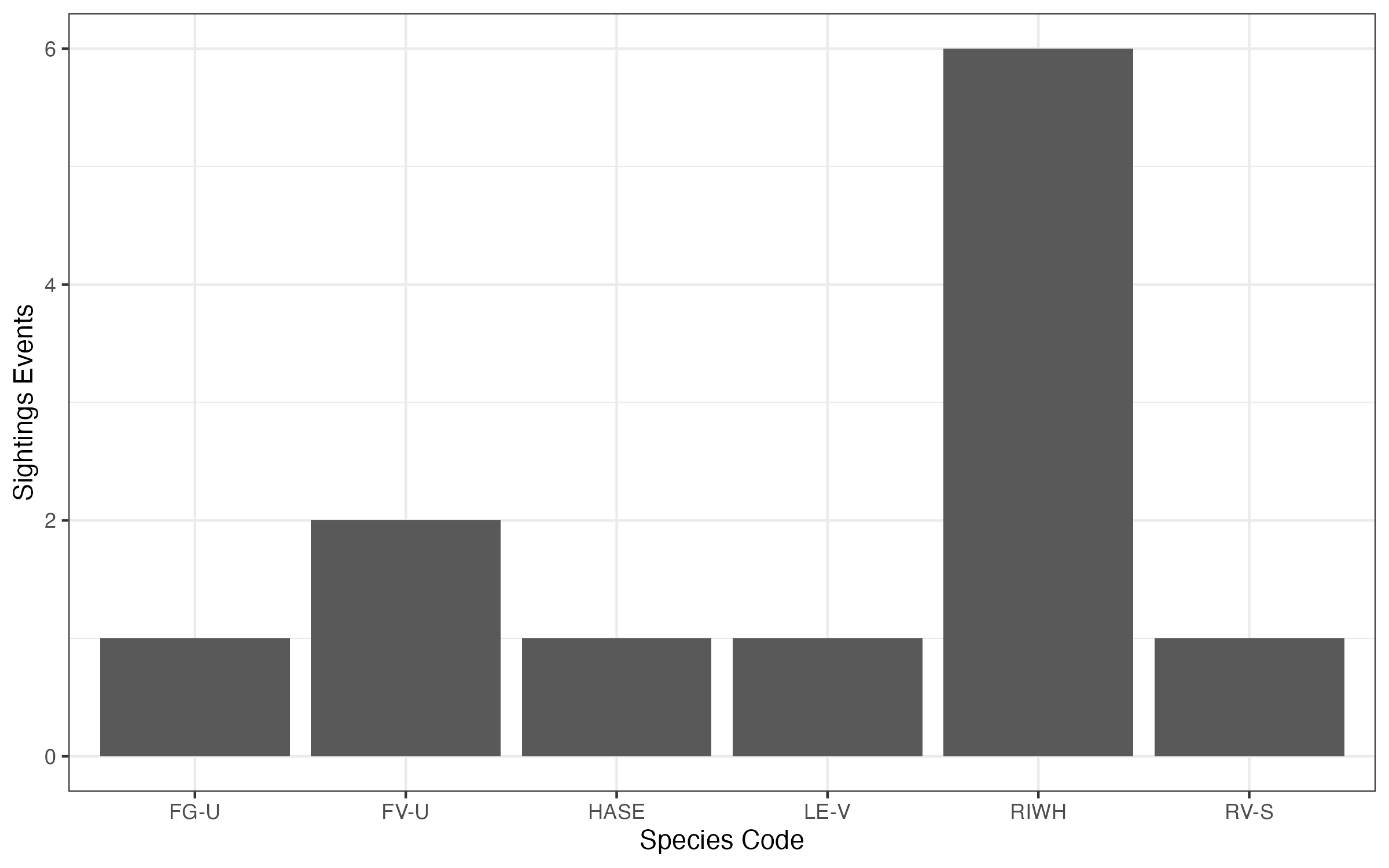

---

4.4 Scatter plot - vessel speed over time

ggplot() +
  geom_path(data = track, aes(x = datetime_edt, y = speed_kts), alpha = 0.6)+
  labs(x = 'Time (EDT)', y = 'Vessel speed (kts)')+
  theme_bw()
  
# ggsave("figures/scatter_plot.png", width = 8, height = 5, dpi = 300)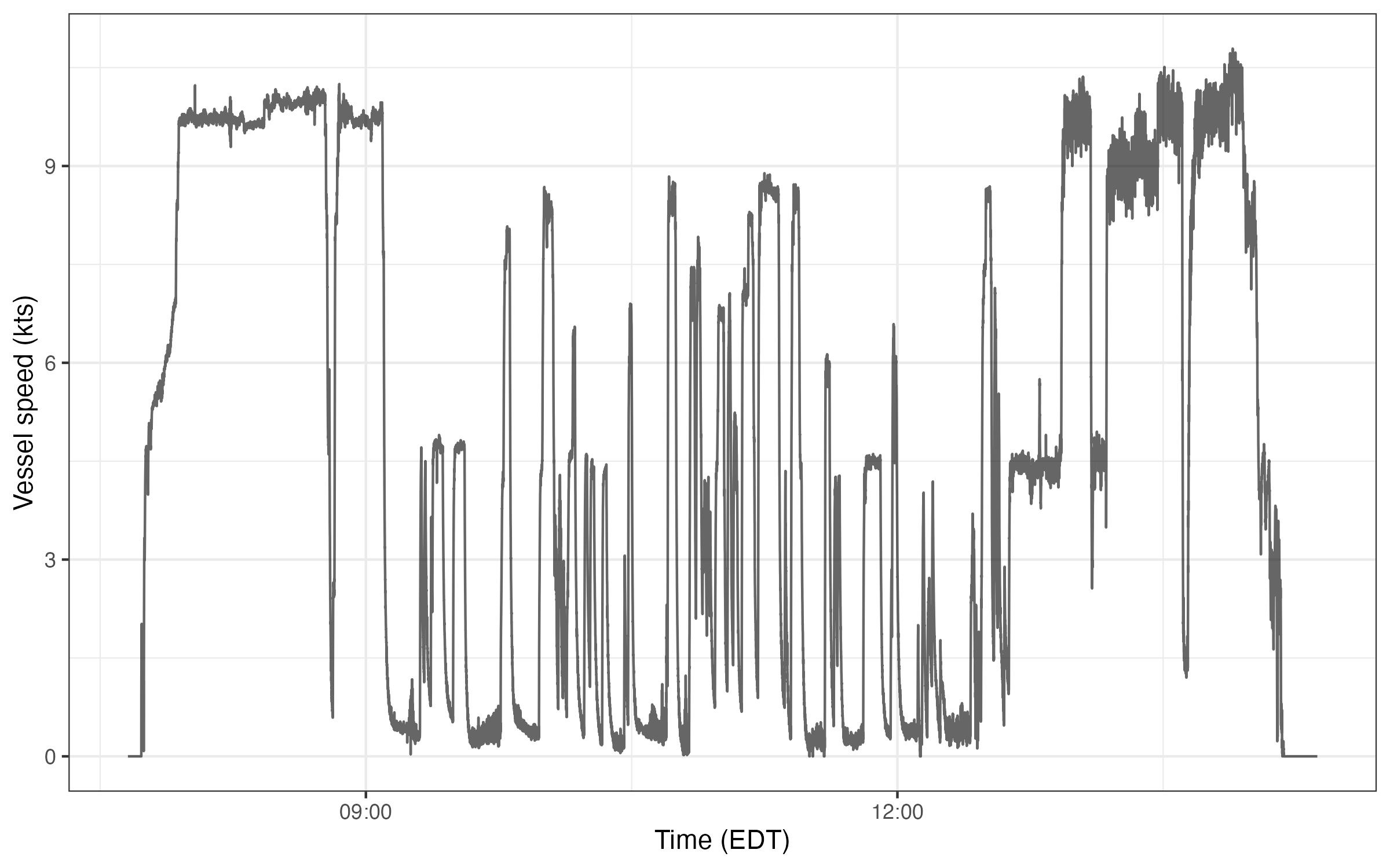

4.5 Survey Maps

4.5.1 Basic map

Plot a quick map of track line and right whale sightings locations:

ggplot() +
  geom_path(data = track, aes(x = longitude, y = latitude), alpha = 0.5)+
  geom_point(data = sightings |> filter(speccode == 'RIWH'), 
             aes(x = longitude, y = latitude), alpha = 0.7)+
  coord_quickmap()+
  labs(x = NULL, 
       y = NULL, 
       title = "Right whale sightings")+
  theme_bw()
  
# ggsave("figures/rw_map.png", width = 8, height = 5, dpi = 300)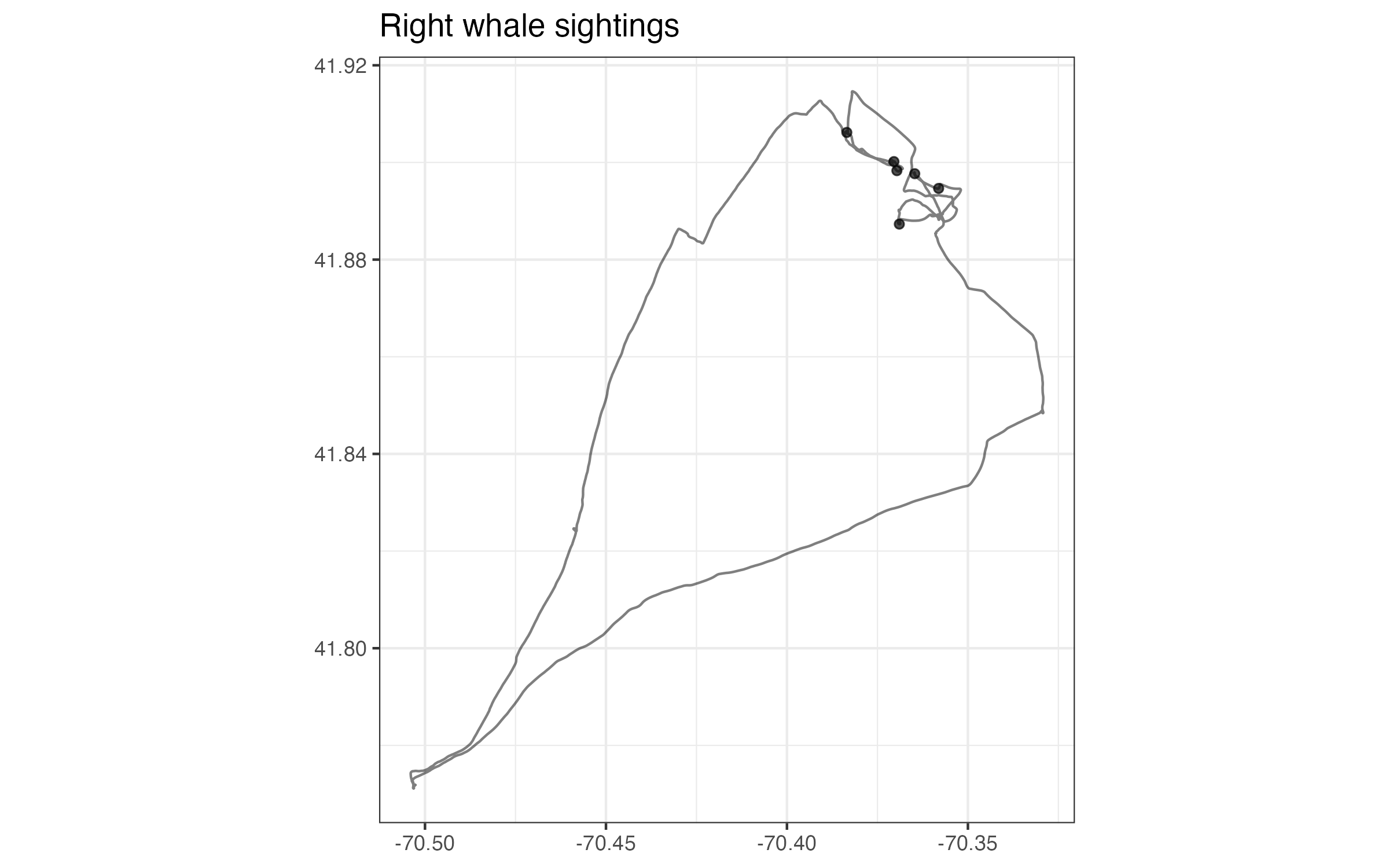

4.5.2 Plotting with sf

Use the sf package to improve mapping functionality. The following is a very simple example to add a coastline.

install.packages(sf)
library(sf)

# import the coastline sf object from my website
coastline_sf <- readRDS(url('https://hansenjohnson.org/files/data/sf-coastline.rds'))

# define the plot limits
buffer = 0.05
min_lon = min(track$longitude, na.rm = T) - buffer
min_lat = min(track$latitude, na.rm = T) - buffer
max_lon = max(track$longitude, na.rm = T) + buffer
max_lat = max(track$latitude, na.rm = T) + buffer

# plot
ggplot() +
  geom_sf(data = coastline_sf) +
  geom_path(data = track, aes(x = longitude, y = latitude), alpha = 0.5) +
  geom_point(data = sightings |> filter(speccode == 'RIWH'), 
             aes(x = longitude, y = latitude), alpha = 0.7) +
  coord_sf(xlim = c(min_lon, max_lon), ylim = c(min_lat, max_lat)) +
  labs(x = NULL, 
       y = NULL, 
       title = "Right whale sightings")+
  theme_bw()

# ggsave("figures/sf_map.png", width = 6, height = 6, dpi = 300)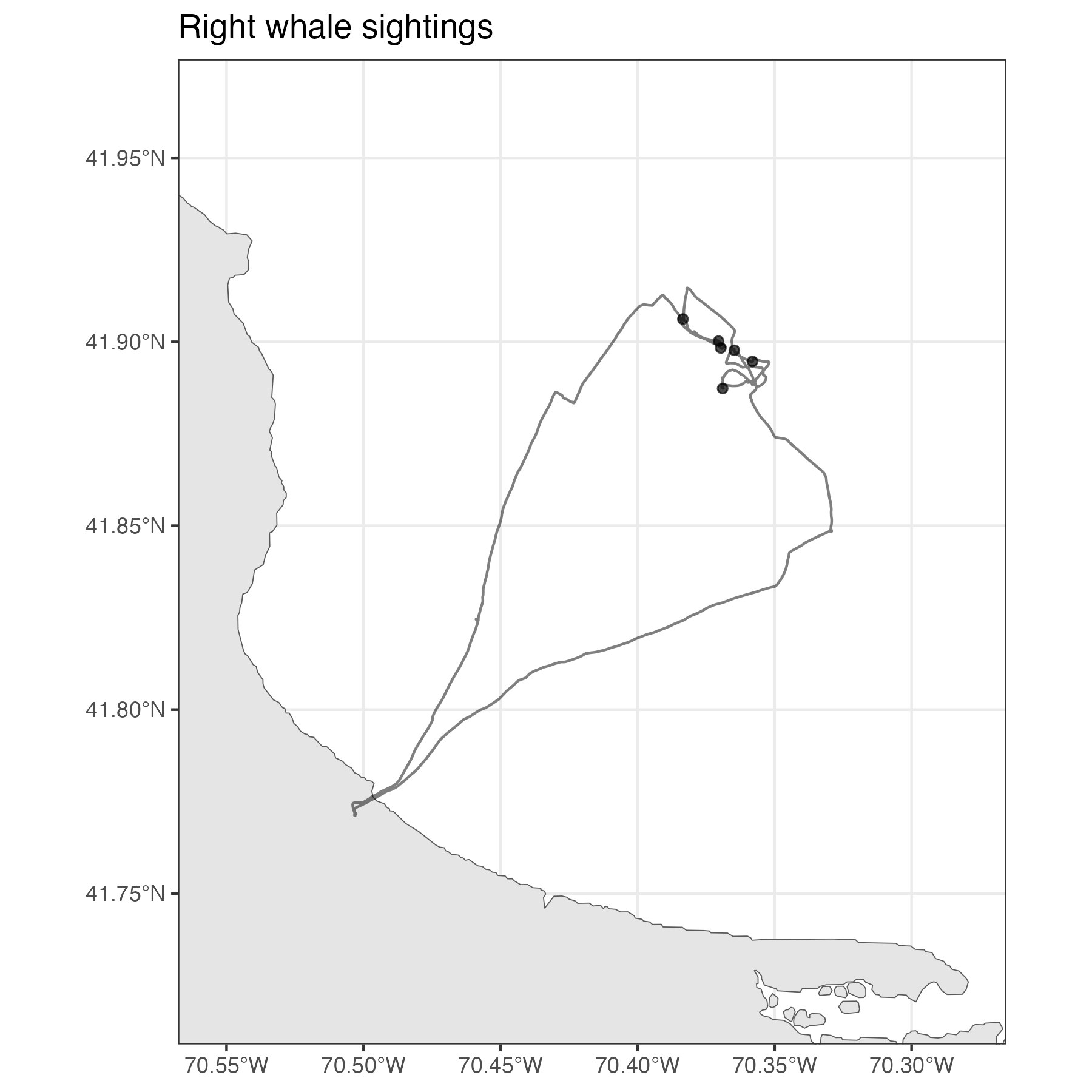

---

4.6 Saving Figures with ggsave()

# Save the last plot
ggsave("figures/survey_map.jpg",
       width = 8, height = 5, dpi = 300)

# Save a named plot object
p <- ggplot() + 
      geom_bar(data = sightings, aes(x = speccode))

ggsave("figures/lame-bar-plot.pdf", plot = p,
       width = 6, height = 4)   # PDFs are vector graphics — no dpi needed

Tip

Create a figures/ folder in your project before saving. For journal submissions use dpi = 300 (PNG) or vector formats (PDF/SVG). width and height are in inches by default.

Bonus: interactive map with leaflet

Use the leaflet package to plot an interactive map.

# Install the package if you haven't already
install.packages("leaflet")

# Load the library
library(leaflet)

# Create an interactive map 
leaflet() |>

  # add tiles
  addProviderTiles("Esri.OceanBasemap") |>
  
  # add lines
  addPolylines(
    data = track,
    lng = ~longitude,
    lat = ~latitude,
    color = 'black',
    weight = 2,
    opacity = 0.6
  ) |>
  
  # add points
  addCircleMarkers(
    data = sightings,
    lng = ~longitude,
    lat = ~latitude,
    radius = 4,
    stroke = FALSE,
    fillOpacity = 0.6,
    popup = ~paste0(
      "Sighting number: ", number, "<br>",
      "Species code: ", speccode, "<br>",
      "Number: ", number, "<br>",
      "Time: ", datetime_edt
    ))

Tip

For more plot examples, check out the ggplot2 tutorial I built several years ago.

Note

Next: Module 5 — Reporting with R Markdown →